Reading Notes: Kimi Delta Attention
Paper: https://arxiv.org/pdf/2510.26692
Code: https://github.com/fla-org/flash-linear-attention
Disclaimer: These are personal reading notes. Some derivations are my own and may be incorrect, so they should be cross-checked against the code later.
Motivation
- improving delta rule with fine-grained gating
Notations
- Bold uppercase letters such as
S and Q denote matrices.
- Symbols like
q_t and k_t denote column vectors with shape [d, 1], while matrices are written in shape [L, d]. Because of this convention, some transpose operations will appear.
- Symbols like
W_t denote learnable parameters.
q_t refers to the t-th row of Q.- \(\square_{[t]} = \square_{[t]}^{1:C} \in \mathbb{R}^{C \times d} \quad\text{for}\quad \square \in \{ \mathbf{Q, K, V,...} \}\)
Background
- Gated Linear Attention
- Online Learning
- DeltaNet and Gated DeltaNet
Kimi Delta Attention
Forward
Comment: Again the WY Representation (i.e. the assumption that P can be written as X - WY) applies here.
The original formulation is simple:
\[\begin{aligned}
\mathbf{S}_t
&= \mathbf{S}_{t-1}
\text{Diag}(\boldsymbol{\alpha}_t)
(\mathbf{I} - \beta_t \boldsymbol{k}_t \boldsymbol{k}_t^\top)
+
\beta_t \boldsymbol{v}_t \boldsymbol{k}_t^\top
\in \mathbb{R}^{d_v \times d_k}
\\
\\
\boldsymbol{o}_t
&= \mathbf{S}_{t}\boldsymbol{q}_t
\end{aligned}\]
Next, following the derivation for DeltaNet, define the chunkwise notation and the following auxiliary quantities:
\[\begin{aligned}
\mathbf{P}_{[t]}^{r} &= \prod_{i=t C + 1}^{t C + r}
\text{Diag}(\boldsymbol{\alpha}_i)
(\mathbf{I} - \beta_{i} \boldsymbol{k}_{i} \boldsymbol{k}_{i}^{\top})
\in \mathbb{R}^{d_k \times d_k}
\\
\\
\mathbf{H}_{[t]}^{r} &= \sum_{i=tC + 1}^{tC + r}
\beta_{i} (\boldsymbol{v}_{i} \boldsymbol{k}_{i}^{\top})
\prod_{j=i + 1}^{t C + r}
\text{Diag}(\boldsymbol{\alpha}_j)
(\mathbf{I} - \beta_{j} \boldsymbol{k}_{j} \boldsymbol{k}_{j}^{\top})
\in \mathbb{R}^{d_v \times d_k}
\end{aligned}\]
Then the chunkwise state can be written as:
\[\begin{aligned}
\mathbf{S}_{[t]}^{r}
=
\mathbf{S}_{[t-1]}^{C}
\mathbf{P}_{[t]}^{r} + \mathbf{H}_{[t]}^{r}
, \quad
\text{where }
\mathbf{S}_{[-1]}^{C} = \mathbf{0}
\end{aligned}\]
On the other hand, suppose that:
\[\begin{aligned}
\mathbf{S}_t = \sum_{i=1}^{t}
\text{Diag}(\boldsymbol{\eta}_t)
\text{Diag}(\boldsymbol{\xi}_i)
\boldsymbol{u}_i
\boldsymbol{k}_i^\top
\text{Diag}(\boldsymbol{\epsilon}_i)
\text{Diag}(\boldsymbol{\gamma}_t)
\end{aligned}\]
Then, by induction, we obtain:
\[\begin{aligned}
\mathbf{S}_t &=
\mathbf{S}_{t-1}
\text{Diag}(\boldsymbol{\alpha}_t)
+ \beta_t \left(
\boldsymbol{v}_t -
\mathbf{S}_{t-1}
\text{Diag}(\boldsymbol{\alpha}_t)
\boldsymbol{k}_t
\right) \boldsymbol{k}_t^\top
\\&=
\sum_{i=1}^{t-1}
\text{Diag}(\boldsymbol{\eta}_{t-1})
\text{Diag}(\boldsymbol{\xi}_i)
\boldsymbol{u}_i
\boldsymbol{k}_i^\top
\text{Diag}(\boldsymbol{\epsilon}_i)
\text{Diag}(\boldsymbol{\gamma}_{t-1})
\text{Diag}(\boldsymbol{\alpha}_{t})
\\&+ \beta_t \left(
\boldsymbol{v}_t -
\sum_{i=1}^{t-1}
\text{Diag}(\boldsymbol{\eta}_{t-1})
\text{Diag}(\boldsymbol{\xi}_i)
\boldsymbol{u}_i
\boldsymbol{k}_i^\top
\text{Diag}(\boldsymbol{\epsilon}_i)
\text{Diag}(\boldsymbol{\gamma}_{t-1})
\text{Diag}(\boldsymbol{\alpha}_{t})
\boldsymbol{k}_t
\right) \boldsymbol{k}_t^\top
\\&=
\sum_{i=1}^{t}
\text{Diag}(\boldsymbol{\eta}_{t})
\text{Diag}(\boldsymbol{\xi}_i)
\boldsymbol{u}_i
\boldsymbol{k}_i^\top
\text{Diag}(\boldsymbol{\epsilon}_i)
\text{Diag}(\boldsymbol{\gamma}_{t})
\end{aligned}\]
after we set
\[\begin{aligned}
\text{Diag}(\boldsymbol{\gamma}_t)
=
\prod_{i=1}^t
\text{Diag}(\boldsymbol{\alpha}_i)
,\quad
\text{Diag}(\boldsymbol{\eta}_t) = \mathbf{I}
,\quad
\text{Diag}(\boldsymbol{\epsilon}_t)
= \text{Diag}(\boldsymbol{\gamma}_t)^{-1}
\end{aligned}\]
then we can easily get
\[\begin{aligned}
\boldsymbol{u}_t
&=
\beta_t
\text{Diag}(\boldsymbol{\xi}_t)^{-1}
\left(
\boldsymbol{v}_t -
\sum_{i=1}^{t-1}
\text{Diag}(\boldsymbol{\xi}_i)
\boldsymbol{u}_i
\boldsymbol{k}_i^\top
\text{Diag}(\boldsymbol{\epsilon}_i)
\text{Diag}(\boldsymbol{\gamma}_{t})
\boldsymbol{k}_t
\right)
\end{aligned}\]
after absorbing \xi into u, we finally get
\[\begin{aligned}
\mathbf{S}_t = \sum_{i=1}^{t} \boldsymbol{u}_i
\left(\text{Diag}(\boldsymbol{\gamma}_i)^{-1} \boldsymbol{k}_i\right)^\top
\text{Diag}(\boldsymbol{\gamma}_t)
,\quad
\boldsymbol{u}_t
&=
\beta_t
\left(
\boldsymbol{v}_t -
\sum_{i=1}^{t-1}
\boldsymbol{u}_i
\left(\text{Diag}(\boldsymbol{\gamma}_i)^{-1} \boldsymbol{k}_i\right)^\top
\left(\text{Diag}(\boldsymbol{\gamma}_{t}) \boldsymbol{k}_t\right)
\right)
\end{aligned}\]
almost the same as in Gated Delta Net.
Meanwhile, the product of Householder transforms of the form (I - beta_t k_t k_t^T) can always be written in a low-rank form using the WY representation. So we further derive this, again using almost the same induction process.
When k = 0, we have
\[\begin{aligned}
\mathbf{P}_{[t]}^{r} = \text{Diag}(\boldsymbol{\gamma}_{[t]}^r)
\end{aligned}\]
So we assume that
\[\begin{aligned}
\mathbf{P}_{[t]}^{r} = \text{Diag}(\boldsymbol{\gamma}_{[t]}^r) - \sum_{i=1}^{r}
\text{Diag}(\boldsymbol{\eta}_{[t]}^r)
\text{Diag}(\boldsymbol{\xi}_{[t]}^i)
\boldsymbol{w}_{[t]}^{i} \boldsymbol{k}_{[t]}^{i \top}
\text{Diag}(\boldsymbol{\epsilon}_{[t]}^i)
\text{Diag}(\boldsymbol{\gamma}_{[t]}^r)
\end{aligned}\]
then we have
\[\begin{aligned}
\mathbf{P}_{[t]}^{r}
&=
\mathbf{P}_{[t]}^{r-1}
\text{Diag}(\boldsymbol{\alpha}_{[t]}^r)
(\mathbf{I} - \beta_{[t]}^r \boldsymbol{k}_{[t]}^r \boldsymbol{k}_{[t]}^{r\top})
\\ \\&=
\text{Diag}(\boldsymbol{\gamma}_{[t]}^r)
-
\text{Diag}(\boldsymbol{\gamma}_{[t]}^r)
\beta_{[t]}^r \boldsymbol{k}_{[t]}^r \boldsymbol{k}_{[t]}^{r\top}
\\ \\&-
\sum_{i=1}^{r-1}
\text{Diag}(\boldsymbol{\eta}_{[t]}^{r-1})
\text{Diag}(\boldsymbol{\xi}_{[t]}^i)
\boldsymbol{w}_{[t]}^{i} \boldsymbol{k}_{[t]}^{i \top}
\text{Diag}(\boldsymbol{\epsilon}_{[t]}^i)
\text{Diag}(\boldsymbol{\gamma}_{[t]}^{r-1})
\\ \\&+
\sum_{i=1}^{r-1}
\text{Diag}(\boldsymbol{\eta}_{[t]}^{r-1})
\text{Diag}(\boldsymbol{\xi}_{[t]}^i)
\boldsymbol{w}_{[t]}^{i} \boldsymbol{k}_{[t]}^{i \top}
\text{Diag}(\boldsymbol{\epsilon}_{[t]}^i)
\text{Diag}(\boldsymbol{\gamma}_{[t]}^{r-1})
\text{Diag}(\boldsymbol{\alpha}_{[t]}^r)
\beta_{[t]}^r \boldsymbol{k}_{[t]}^r \boldsymbol{k}_{[t]}^{r\top}
\end{aligned}\]
By canceling identical terms, setting the parameters as follows and absorbing \xi to w, we have
\[\begin{aligned}
\text{Diag}(\boldsymbol{\gamma}_{[t]}^i)
&=
\prod_{j=1}^i
\text{Diag}(\boldsymbol{\alpha}_{[t]}^j)
,\quad
\text{Diag}(\boldsymbol{\eta}_{[t]}^i) = \mathbf{I}
,\quad
\text{Diag}(\boldsymbol{\epsilon}_{[t]}^i)
= \text{Diag}(\boldsymbol{\gamma}_{[t]}^i)^{-1}
\\
\\
\boldsymbol{w}_{[t]}^{r}
&=
\beta_{[t]}^r
\left(\mathbf{I} -
\sum_{i=1}^{r-1}
\boldsymbol{w}_{[t]}^{i}
\left(
\text{Diag}(\boldsymbol{\gamma}_{[t]}^i)^{-1}
\boldsymbol{k}_{[t]}^{i}
\right)^\top
\right)
\text{Diag}(\boldsymbol{\gamma}_{[t]}^r)
\boldsymbol{k}_{[t]}^r
\\
\\
\mathbf{P}_{[t]}^{r} &=
\left(\mathbf{I}- \sum_{i=1}^{r}
\boldsymbol{w}_{[t]}^{i}
\left(
\text{Diag}(\boldsymbol{\gamma}_{[t]}^i)^{-1}
\boldsymbol{k}_{[t]}^{i}
\right)^\top
\right)
\text{Diag}(\boldsymbol{\gamma}_{[t]}^r)
\end{aligned}\]
Substituting this into the chunkwise recurrence gives:
\[\begin{aligned}
\mathbf{S}_{[t]}^{r}
&=
\mathbf{S}_{[t-1]}^{C}
\left(\mathbf{I}- \sum_{i=1}^{r}
\boldsymbol{w}_{[t]}^{i}
\left(
\text{Diag}(\boldsymbol{\gamma}_{[t]}^i)^{-1}
\boldsymbol{k}_{[t]}^{i}
\right)^\top
\right)
\text{Diag}(\boldsymbol{\gamma}_{[t]}^r)
\\&+
\sum_{i=1}^{r} \boldsymbol{u}_{[t]}^i
\left(
\text{Diag}(\boldsymbol{\gamma}_{[t]}^i)^{-1}
\boldsymbol{k}_{[t]}^i\right)^\top
\text{Diag}(\boldsymbol{\gamma}_{[t]}^r)
\\&=
\mathbf{S}_{[t-1]}^{C}
\text{Diag}(\boldsymbol{\gamma}_{[t]}^r)
+
\sum_{i=1}^{r}
\left(
\boldsymbol{u}_{[t]}^i
-
\mathbf{S}_{[t-1]}^{C}
\boldsymbol{w}_{[t]}^{i}
\right)
\left(
\text{Diag}(\boldsymbol{\gamma}_{[t]}^i)^{-1}
\boldsymbol{k}_{[t]}^{i}
\right)^\top
\text{Diag}(\boldsymbol{\gamma}_{[t]}^r)
\\
\\
\boldsymbol{o}_{[t]}^{r}
&=
\mathbf{S}_{[t]}^{r} \boldsymbol{q}_{[t]}^{r}
\\ \\&=
\mathbf{S}_{[t-1]}^{C}
\left(
\text{Diag}(\boldsymbol{\gamma}_{[t]}^r)
\boldsymbol{q}_{[t]}^{r}
\right)
+
\sum_{i=1}^{r}
\left(
\boldsymbol{u}_{[t]}^i
-
\mathbf{S}_{[t-1]}^{C}
\boldsymbol{w}_{[t]}^{i}
\right)
\left(
\text{Diag}(\boldsymbol{\gamma}_{[t]}^i)^{-1}
\boldsymbol{k}_{[t]}^{i}
\right)^\top
\left(
\text{Diag}(\boldsymbol{\gamma}_{[t]}^r)
\boldsymbol{q}_{[t]}^{r}
\right)
\end{aligned}\]
Now define:
\[\begin{aligned}
\mathbf{\Gamma}_{[t]} &= [
\boldsymbol{\gamma}_{[t]}^1,
\boldsymbol{\gamma}_{[t]}^2,
...,
\boldsymbol{\gamma}_{[t]}^C
]^\top
\\
\\
\overleftarrow{\square_{[t]}}
&=
\square_{[t]}
\odot
\mathbf{\Gamma}_{[t]}
,\quad
\overrightarrow{\square_{[t]}}
=
\square_{[t]}
\oslash
\mathbf{\Gamma}_{[t]}
\quad\text{for}\quad \square \in \{ \mathbf{Q}, \mathbf{K}, \mathbf{W}\}
\end{aligned}\]
Then we can rewrite the computation in matrix form as (kind reminder: do not forget to transpose on O):
\[\begin{aligned}
\mathbf{S}_{[t]}^{C}
&=
\mathbf{S}_{[t-1]}^{C}
\text{Diag}(\boldsymbol{\gamma}_{[t]}^C)
+
\left(\mathbf{U}_{[t]}^\top - \mathbf{S}_{[t-1]}^{C} \mathbf{W}_{[t]}^\top \right)\overrightarrow{\mathbf{K}_{[t]}}
\text{Diag}(\boldsymbol{\gamma}_{[t]}^C)
\\
\\
\mathbf{O}_{[t]}
&=
\overleftarrow{\mathbf{Q}_{[t]}} \mathbf{S}_{[t-1]}^{C \top}
+
\left( \overleftarrow{\mathbf{Q}_{[t]}} \overrightarrow{\mathbf{K}_{[t]}}^\top \odot \mathbf{M} \right) \left(\mathbf{U}_{[t]} - \mathbf{W}_{[t]} \mathbf{S}_{[t-1]}^{C \top} \right)
\end{aligned}\]
Comment: This form is natural, and the derivation proves the power of DeltaNet once again.
Next, we turn to u_[t] and w_[t]. Here, M_{-1} = M - I denotes the strictly lower-triangular mask with zeros on the diagonal.
Starting from the recurrence for u_[t], we get:
\[\begin{aligned}
\boldsymbol{u}_{[t]}^r
&=
\beta_{[t]}^r
\left(
\boldsymbol{v}_{[t]}^r -
\sum_{i=1}^{r-1}
\boldsymbol{u}_{[t]}^i
\left(\text{Diag}(\boldsymbol{\gamma}_{[t]}^i)^{-1} \boldsymbol{k}_{[t]}^i\right)^\top
\left(\text{Diag}(\boldsymbol{\gamma}_{[t]}^r) \boldsymbol{k}_{[t]}^r\right)
\right)
\\
\\
\Rightarrow
\mathbf{U}_{[t]}
&=
\text{Diag}(\boldsymbol{\beta}_{[t]})
\left(
\mathbf{V}_{[t]} -
\left(
\overleftarrow{\mathbf{K}_{[t]}}
\overrightarrow{\mathbf{K}_{[t]}}^\top
\odot
\mathbf{M}_{-1}
\right)
\mathbf{U}_{[t]}
\right)
\\
\\
\Rightarrow
\mathbf{U}_{[t]}
&=
\left(
\mathbf{I} +
\text{Diag}(\boldsymbol{\beta}_{[t]})
\left(
\overleftarrow{\mathbf{K}_{[t]}}
\overrightarrow{\mathbf{K}_{[t]}}^\top
\odot
\mathbf{M}_{-1}
\right)
\right)^{-1}
\text{Diag}(\boldsymbol{\beta}_{[t]})
\mathbf{V}_{[t]}
\end{aligned}\]
By the same argument, we also have:
\[\begin{aligned}
\mathbf{W}_{[t]}
=
\left(
\mathbf{I} +
\text{Diag}(\boldsymbol{\beta}_{[t]})
\left(
\overleftarrow{\mathbf{K}_{[t]}}
\overrightarrow{\mathbf{K}_{[t]}}^\top
\odot \mathbf{M}_{-1}
\right) \right)^{-1}
\text{Diag}(\boldsymbol{\beta}_{[t]})
\overleftarrow{\mathbf{K}_{[t]}}
\end{aligned}\]
Therefore, in order to compute U_[t] and W_[t], the key quantities are:
\[\begin{aligned}
\mathbf{\widetilde{A}}_{[t]}
=
\left(\mathbf{I} + \text{Diag}(\boldsymbol{\beta}_{[t]}) \left( \overleftarrow{\mathbf{K}_{[t]}} \overrightarrow{\mathbf{K}_{[t]}}^\top \odot \mathbf{M}_{-1} \right) \right)^{-1}
\end{aligned}\]
The matrix inversion step can be handled in the same way as in the DeltaNet notes.
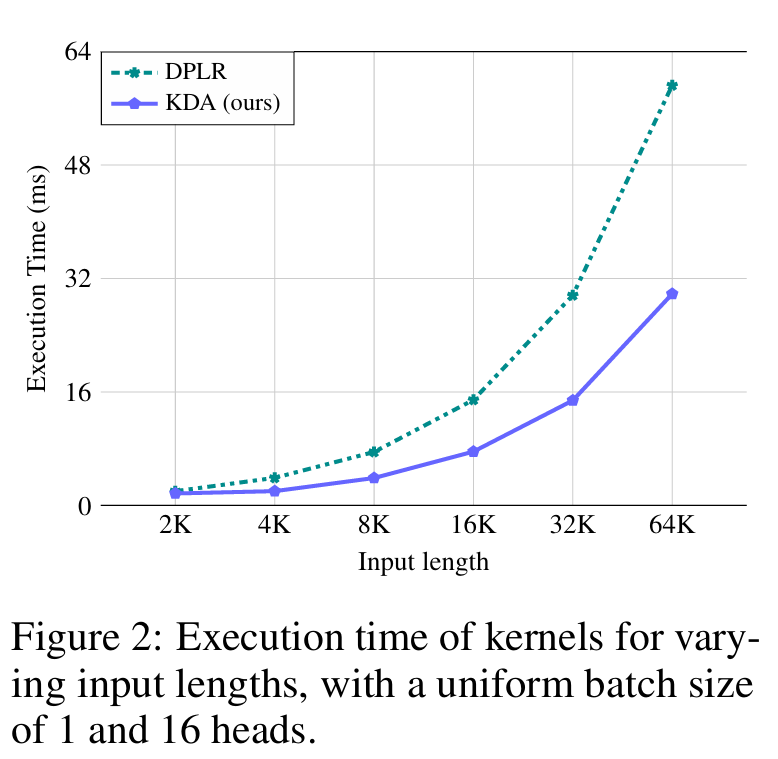
Compare to DPLR
compared to DPLR:
$\(\begin{aligned}
\mathbf{S}_t
&= \mathbf{S}_{t-1}
(\text{Diag}(\boldsymbol{\alpha}_t) - \boldsymbol{b}_t \boldsymbol{a}_t^\top)
+
\beta_t \boldsymbol{v}_t \boldsymbol{k}_t^\top
\in \mathbb{R}^{d_v \times d_k}
\end{aligned}\)$
Comment: Prior works like GLA have addressed that when interacting with the decay parameter Diag, one must be highly mindful of numerical precision. It is better to use secondary chunking in full precision, which trades speed for stability. n DPLR, this may lead to four numerically fragile terms, i.e. Q @ K, Q @ B, A @ B, A @ K. KDA binds both variables a and b to k, reducing this to only two terms, i.e. Q * K, K @ K.
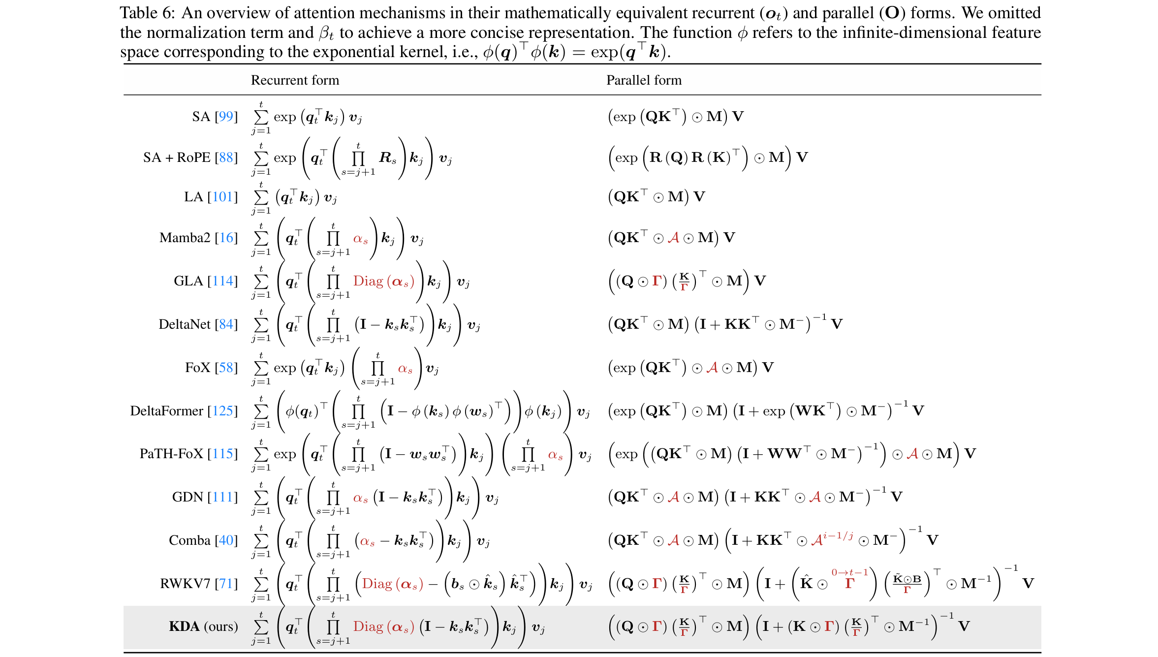
Compare to Other Models
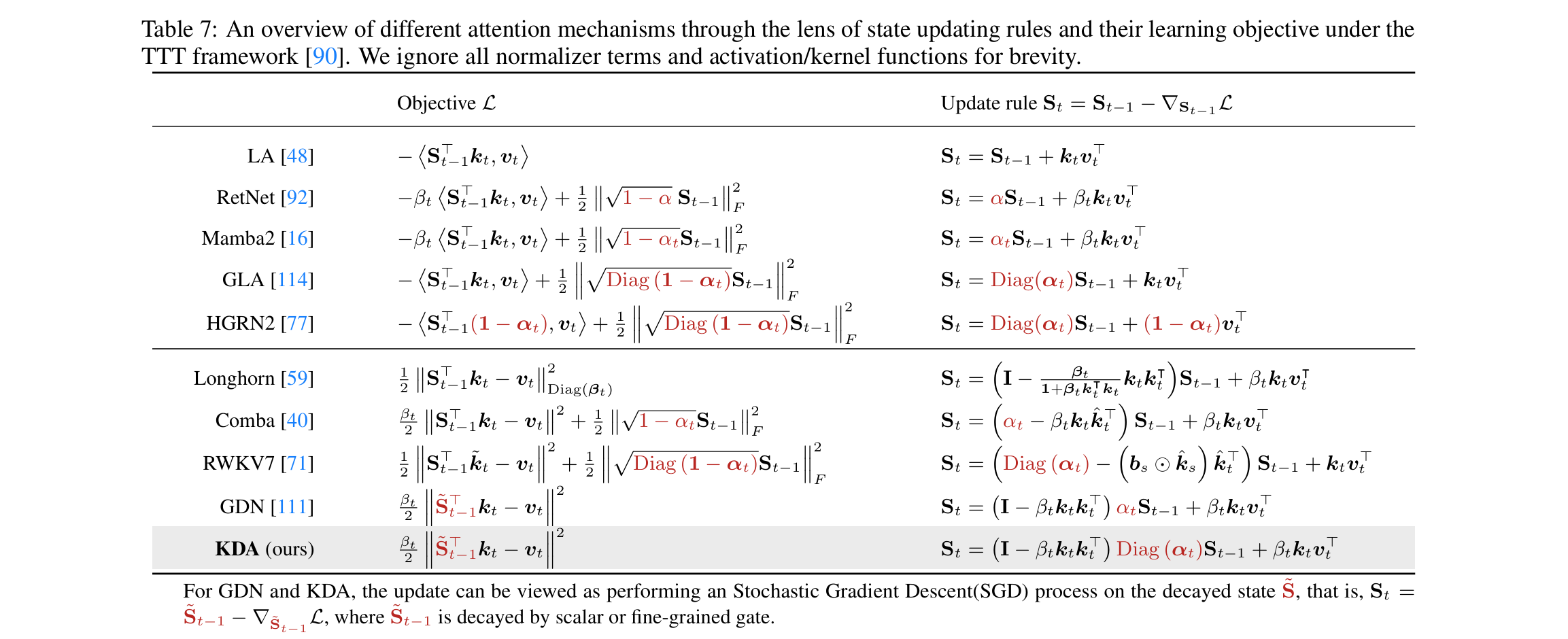
Test time training perspective
Model Architecture

- KDA layer
\[\begin{aligned}
\boldsymbol{q}_{t}^{h}, \boldsymbol{k}_{t}^{h}
&= \operatorname{L2Norm}\left(\operatorname{Swish}\left(\operatorname{ShortConv}\left(\mathbf{W}_{q / k}^{h} \boldsymbol{x}_{t}\right)\right)\right) \in \mathbb{R}^{d_{k}}
\\
\\
\boldsymbol{v}_{t}^{h}
&=\operatorname{Swish}\left(\operatorname{ShortConv}\left(\mathbf{W}_{v}^{h} \boldsymbol{x}_{t}\right)\right) \in \mathbb{R}^{d_{v}}
\\
\\
\alpha_{t}^{h} &=f\left(\mathbf{W}_{\alpha}^{\uparrow} \mathbf{W}_{\alpha}^{\downarrow} \boldsymbol{x}_{t}\right) \in[0,1]^{d_{k}}
\\
\\
\beta_{t}^{h}
&=\operatorname{Sigmoid}\left(\mathbf{W}_{\beta}^{h} \boldsymbol{x}_{t}\right) \in[0,1]
\\
\\
\boldsymbol{o}_{t}
&=\mathbf{W}_{o}\left(\operatorname{Sigmoid}\left(\mathbf{W}_{g}^{\uparrow} \mathbf{W}_{g}^{\downarrow} \boldsymbol{x}_{t}\right) \odot \operatorname{RMSNorm}\left(\operatorname{KDA}\left(\boldsymbol{q}_{t}, \boldsymbol{k}_{t}, \boldsymbol{v}_{t}, \boldsymbol{\alpha}_{t}, \beta_{t}\right)\right)\right)
\end{aligned}\]
The gate \(\alpha_t^h\) is computed as \alpha_t^h = -exp(A_log) * softplus(W^up W^down x + dt_bias) which is similar to mamba. A_log has shape [H] and dt_bias has shape [H * K].
- Inter Layer Hybrid
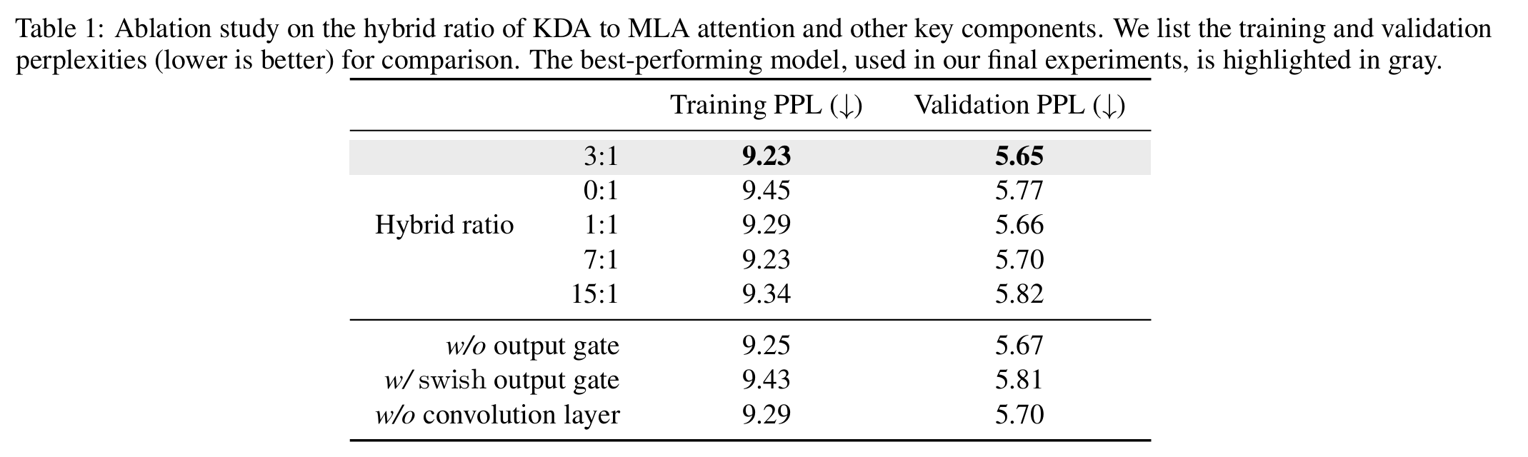
Kimi Linear uses 3:1 KDA: MLA. The main reason for choosing inter-layer rather than intra-layer hybridization (e.g., dynamic routing per head) is infrastructure simplicity.
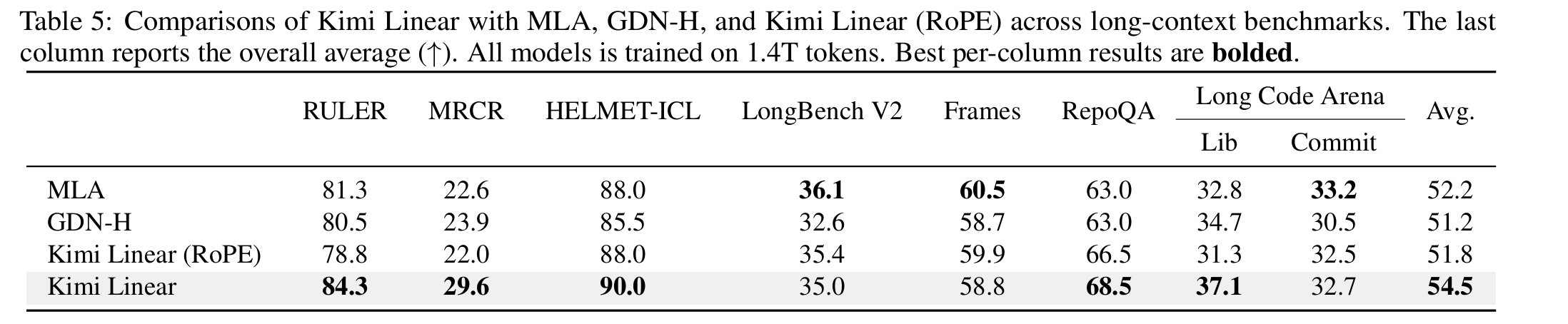
- Use NoPE for MLA
MLA uses NoPE (No Positional Encoding) because KDA inherently captures positional information through its recurrent decay mechanism. This design is also beneficial for long-context extrapolation.
Experiments
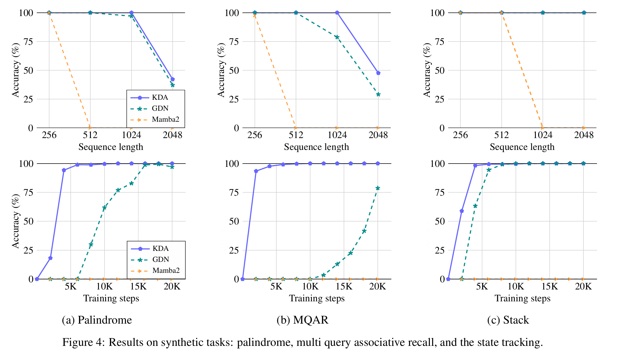
Synthetic tests
Palindrome Generate the reversal

Multi Query Associative Recall (MQAR) Recall the next

Stack stack operations with LIFO.
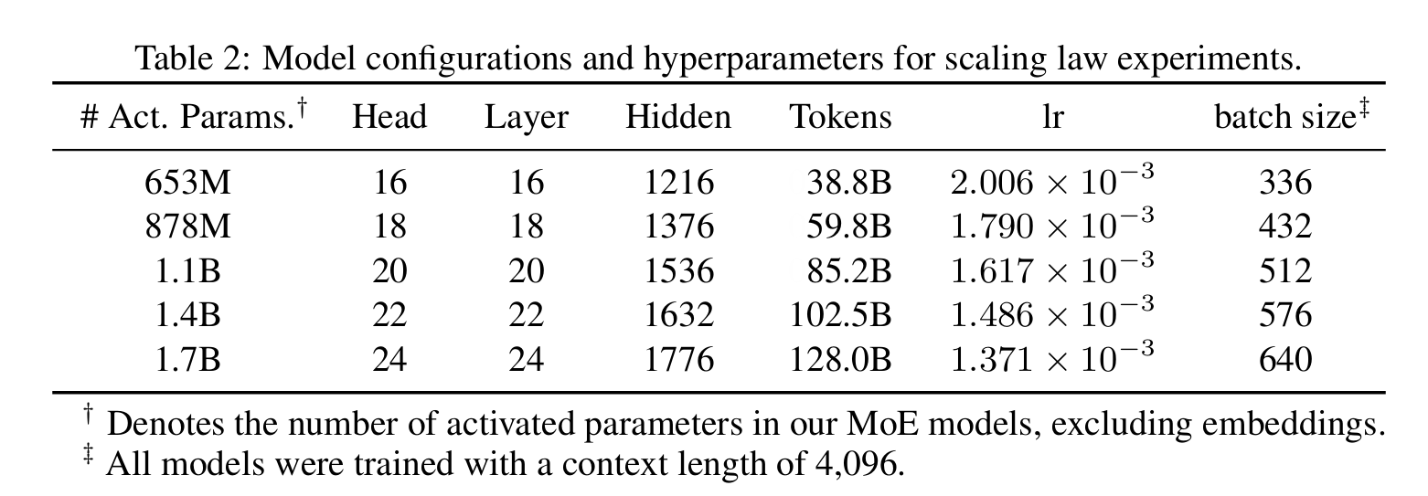
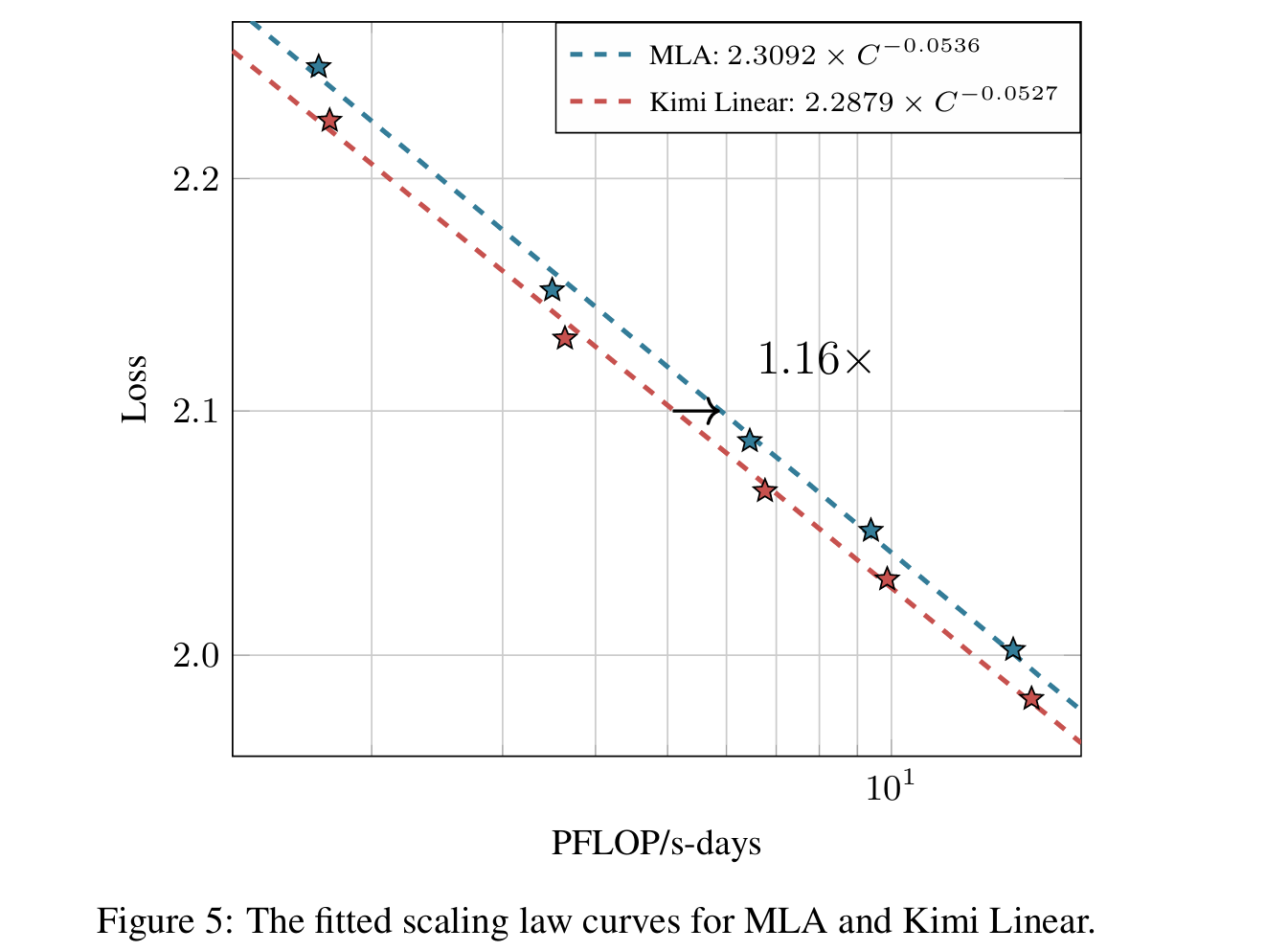
Scaling law
- Base: MoE Moonlight Architecture
- 8 activate / 64 total experts
- Muon Optimizer
- Use Chinchilla scaling law methodology
Language Modeling
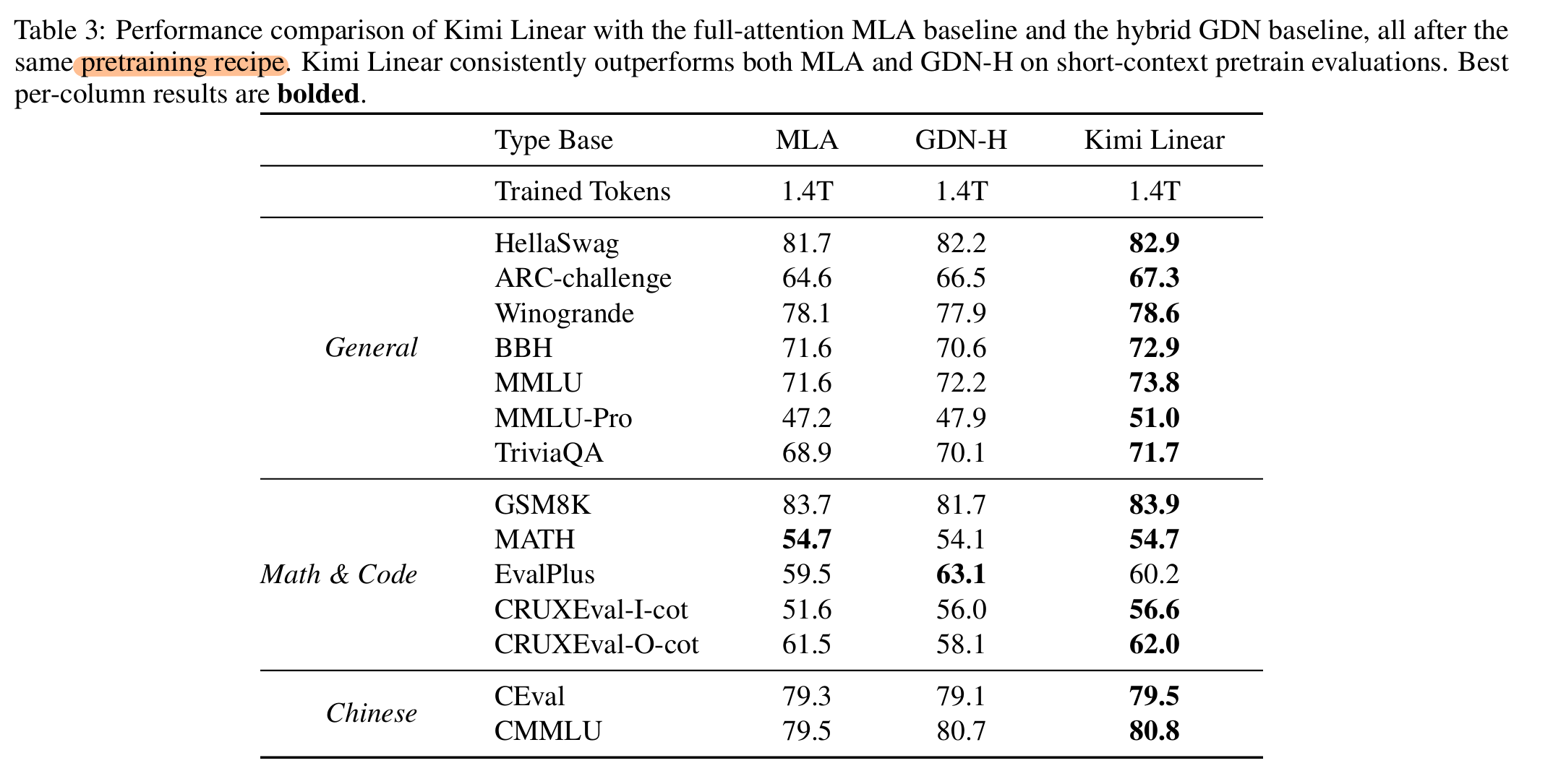
Pre-Training
- Base MoE Moonlight
- 8 activate / 256 total experts with one shared expert
- 48B-A8B
- 4096 context window
- Muon Clip optimizer
- WSD learning rate schedule
- 1.4T tokens from K2 pretraining corpus
- learning rate is set to 1.1 × 10⁻³
- global batch size is fixed at 32 million tokens
- same annealing schedule and long-context activation phase established in Kimi K2
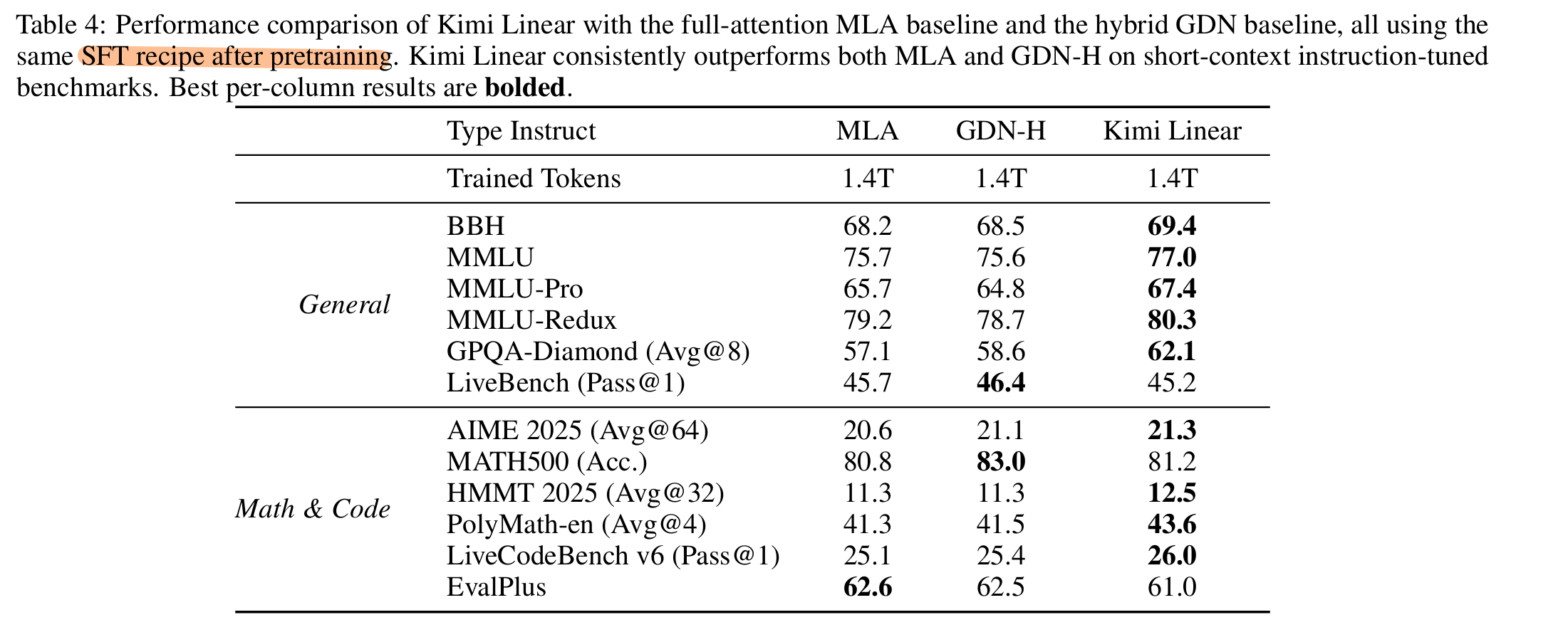
Post-training: SFT
- Kimi K2 SFT data + additional reasoning tasks
- multi-stage SFT approach: initially for general instruction-following, followed by reasoning-intensive data
-
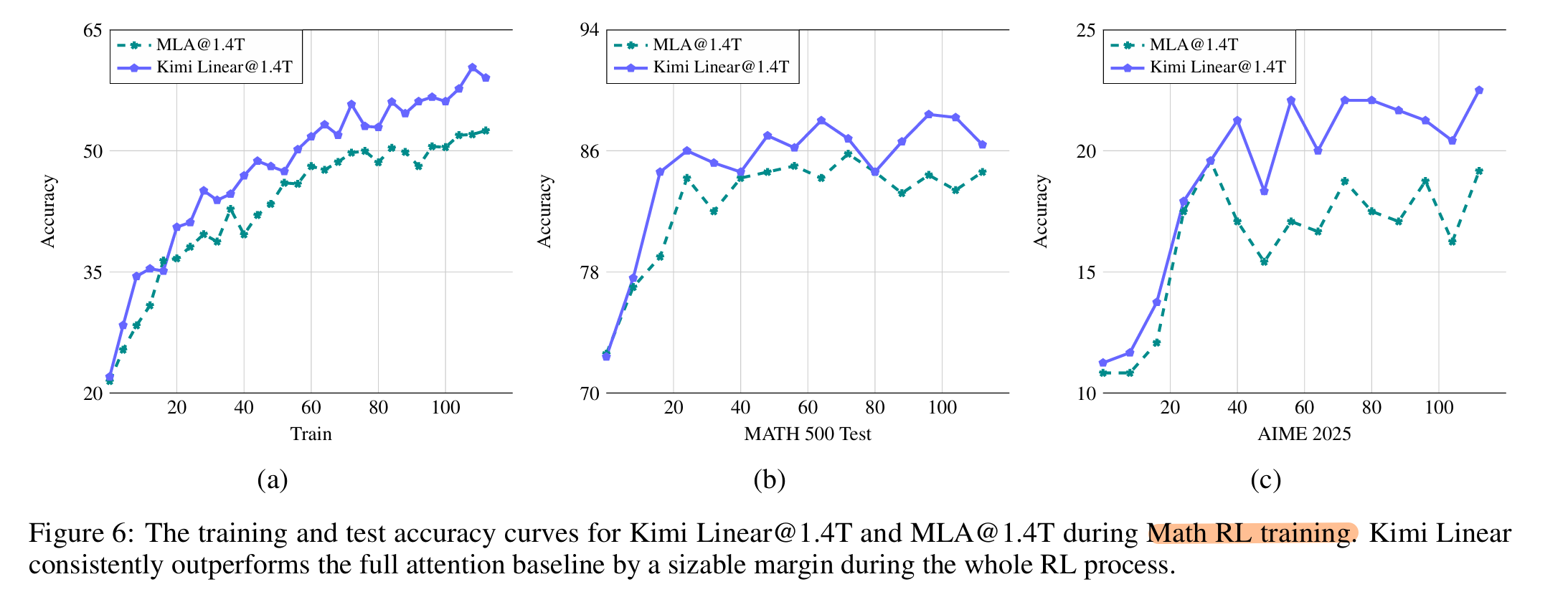
Post-training: RL
- mathematics, code, and STEM from Kimi K2 Data, selected to be of moderate difficulty for the starting checkpoint.
- additional PTX loss. PTX dataset spans both reasoning and general-purpose tasks.
[Warning] Post-training: RL
the precision mismatch between training and inference engines may lead to unstable RL learning
-> truncated importance sampling, dynamically adjust the KL penalty and the mini batch size
Evaluation
- Language Understanding and Reasoning: Hellaswag, ARC-Challenge, Winogrande, MMLU, TriviaQA, MMLU-Redux, MMLU-Pro, GPQA-Diamond, BBH, Livebench.
- Code Generation: LiveCodeBench v6, EvalPlus
- Math&Reasoning: AIME 2025, MATH 500, HMMT 2025, PolyMath-en.
- Long-context: MRCR 5 , RULER, Frames, HELMET-ICL, RepoQA, Long Code Arena, LongBench v2.
- Chinese Language Understanding and Reasoning: C-Eval, and CMMLU.
- Temprature=1.0, LM-Harness-Evaluation
- PPL-based evaluation for MMLU, MMLU-Redux, GPQA-Diamond, and C-Eval with Base Model, Generation Based for others.